EXCEL: Computing Depreciation, Ensuring Quality Performance

 

QUALITY WORK IN COMPUTING DEPRECIATION

The family of depreciation functions includes both the straight-line approach and the accelerated methods, declining balance and sum of years digits.

Excel has the following depreciation functions:

• SLN. Short for "straight line." You know what this one does: it divides the depreciable value of an asset equally across its useful life.

• SYD. Short for "sum of years' digits." The most basic of the accelerated depreciation functions.

• DB. Short for "declining balance." The accounting literature often refers to this as "double declining balance," and the DB function can work in this way.

• DDB. Short for "double declining balance." Again, it is possible to use this function in the usual way, to double the straight-line rate, but you can optionally supply other rates.

The depreciation functions take just a few arguments, which must be listed in a specific order, and not all the arguments are required. The arguments common to all the depreciation functions include the following:

• Cost. The original book value of the asset you're depreciating. Required by all depreciation functions.

·         Salvage. Excel uses the term "salvage" in place of "residual," and to avoid confusion this chapter does the same. The value of the asset at the end of the final depreciation period. Required by all depreciation functions.

• Life. The number of accounting periods, normally years, over which the asset is to be depreciated. Required by all depreciation functions.

• Period. The period for which the depreciation is to be calculated. Required by all the depreciation functions, except SLN (which by definition returns a constant figure regardless of period).

In this context, "required argument" does not mean that you have to supply a value. It does mean that you have to account for it.

For example, =SLN(1000,0,5)

specifies a Cost of 1000, a Salvage of 0 and a Life of 5. An equivalent usage is

=SLN(1000,,5),

which does not supply a Salvage value but accounts for it by means of two consecutive commas. The Salvage argument would normally go there, but because it's missing Excel assumes that Salvage is 0.

 1.    STRAIGHT LINE METHOD

The SLN function returns the amount of depreciation to take in each period. It con[1]forms to the usual tax regulations in requiring that you supply a salvage value that is subtracted from the original book value before calculating the depreciation.

The SLN function syntax is:

=SLN(Cost, Salvage, Life)

Figure 1 below shows how you might lay out a worksheet to give names to cells and make it easier to enter and edit the values of the three arguments, whether you decide to use the function wizard or to enter the function and its arguments directly on the worksheet.

Accelerated Depreciation

Besides straight-line depreciation, Excel provides for four methods of accelerated depreciation. Accelerated depreciation front-loads the depreciation in the earlier periods of an asset's useful life. The rationale is part cupidity and part logic.

As to greed: we usually like to depreciate greater amounts earlier.

As to logic: it's just an extension of the matching principle. To the degree possible, costs should appear in the same accounting period as the benefits they bring to a company. Other things being equal, the newer an asset, the greater benefit it offers. Therefore, the greater portion of the asset's cost should also be recognized earlier.

The Excel functions that accelerate depreciation beyond a straight line are SYD,DB and DDB.

2. SUM-OF-THE-YEARS-DIGITS

The most straightforward of the accelerated depreciation methods is SYD, sum of years' digits. Figure 2 shows how you might set up the worksheet to take advantage of the SYD function.

Like the straight-line approach, the sum of years' digits method requires that you apply the depreciation factor to the asset's depreciable value – the difference between the original cost and the salvage value. The syntax for the SYD function is:

=SYD (Cost, Salvage, Life, Per)

 

3. DECLINING BALANCE

In the traditional method of calculating declining balance depreciation, the straight[1]line rate is doubled. If an asset is judged to have a useful life of four periods, the straight-line method would depreciate it at 25% per period; 25% would be applied to the difference between the cost and the salvage in each period.

The syntax of the DB function is:

=DB(Cost, Salvage, Life, Period, Month)

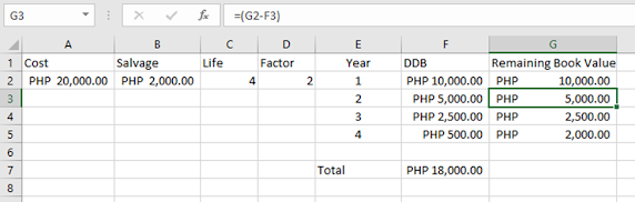
4. DOUBLE-DECLINING BALANCE

I have better news regarding Excel's DDB function than I did regarding its DB function – and it's not limited to the fact that the Period argument in DDB is Period instead of Per.

The DDB function allows you to specify a particular rate of depreciation, with reference to the SLN rate. That is, you can specify a Factor argument that is multi[1]plied by the SLN rate, which is determined by the asset's useful life. (DDB is short for double declining balance.)

In contrast to the DB function, the rate of depreciation used by DDB is not determined by the salvage value. It is determined by dividing the Factor argument by the asset's useful life.

Furthermore, the DDB function does not base periodic depreciation on the asset's original cost less a salvage value – in fact, the only reason that the DDB function takes a Salvage argument is to determine when to stop calculating depreciation.

Here's DDB's full syntax:

=DDB(Cost,Salvage,Life,Period,Factor)

Now you learn how to compute Depreciation, remember it is very important in your business because depreciation is an expense and accounting entails how much value your business assets lose every year. Remember depreciation as a loss and must be subtracted from your revenue. 

Computing depreciation helps the business to cover the total cost of an asset over its lifespan instead of immediately recovering the purchase cost which would see one large cost and lower profits. 

QUARTILE Function in Excel: Focus on Operating Profit

 QUARTILE Function is very simple to use. Let us now see how to use the TILE function in Excel with the help of this example.

Let us focus on Operating Profit.

Here, we will calculate the minimum value, First Quartile, Second Quartile, Third Quartile, and Maximum value by using the QUARTILE Function. We will take the value of the second argument QUART from 0-4 of the QUARTILE function like the below screenshot for this calculation.

Now we will apply the QUARTILE function to the OPERATING PROFIT data.

We will calculate the QUARTILE function for all values one by one by selecting the values from a drop-down list.

Similarly, we will find other values. The final result is shown below:

QUARTILE Function divides the dataset into 4 equal parts.

1st quartile value is 2308, 2nd quartile value is 5055, and 3rd quartile value is 6242.

KPI IN EXCEL : Focus on Operating Profit %

 Key performance indicators (KPIs) are visual measures of performance and usually included in reports. Supported by a specific calculated field, a KPI is designed to help users quickly evaluate the current value and status of a metric against a defined target. 

In this blog, we will use Operating Profit % as a KPI since Small and Medium enterprises need to understand that Operating profit is a useful and accurate indicator of a business's health.

Here's how to use KPI in Excel. Open the data "KPI Data" from Github  https://github.com/alcadelina/KPI

Step 1. Open an Excel file. Click on the File tab on the uppermost ribbon. Go to Options.

Step 2: Under Options > Click on Add-ins. You’ll be able to see the screen as shown below.

Step 3: Select COM Add-ins under the Manage section dropdown and click on the Go button.

Step 4: As soon as you hit the Go button, the COM Add-ins dialog box will pop up. Select Microsoft Power Pivot for Excel from the list of add-ins and click OK.

After enabling this PowerPivot add-in, you should be able to see the PowerPivot option tab on the topmost panel ribbon in your excel.

Step 5: Under the PowerPivot tab in your excel file, click on Manage.

Step 6: It should open a new tab named Power Pivot for Excel. 
Step 7: Once you click on the “From Other Sources” tab, a new window named Table Import Wizard will pop up. There you can see a lot of options from where you can import the data to PowerPivot. Select the Excel file, then click on the Next button to proceed further.

Step 8: Browse the path on where your excel data file is stored and click the Next button to finish the Import.

Step 9: Click on the Finish button once the data table is loaded into PowerPivot.

Step 10: After a successful import, you will be able to see the data as below.

Step 11: Now, in order to create a KPI report, we need to slice and dice our data under the pivot table. Click on the Pivot Table tab under PowerPivot. Once you click it, a new window named Create PivotTable will appear in which you have to select the data from PowerPivot, and it asks you whether you want a pivot table under a new sheet or on the same sheet. I will prefer to go with the same sheet and then will provide the range on which the pivot table should be added. Click OK once done.

Step 12: Select the data under rows, columns, and values, as shown below.

Here we have selected data in the following order:

Rows: Accounting Date Year & Quarter

Values: Sum of Total Sales & Operating Profit

Step 13: Now, we are going to add a calculated column in the pivot. Select Measures under excel sheet. Click on New Measures.

A new window called Measure will pop up. It will allow you to formulate a measure and add it under your pivot table created.

Step 14: Under ” Measure name:”, add a name OPERATING PROFIT %. If you want to add a description for the same, you can add it there as well under the Description section. In this case, Operating Profit Percentage measures how much of a profit the company is generating from their main operations. The operating profit percentage represents the percentage of a company’s sales that ultimately end up as profit. 

Under the Formula section, add the formula =[Sum of Operating Profit]/[Sum of Total Sales] as shown below. It will calculate the OPERATING PROFIT % for you. See the screenshot below.

Above, we have created a new calculated column named Operating Profit %, which can be formulated as the ratio of two columns, Sum of Operating Profit and Sum of Total Sales. 

Step 15: Select the entire column, Operating Profit %, and convert it to % using number formatting.

Step 16: Now our data is ready for KPI’s to be added. Click on the KPIs tab as shown in the figure. Select the New KPI option.

A KPI window will pop up, as shown below. It has some by default values, which we are going to change.

Step 17: In this window, define an Absolute Value for the target as 1. We are doing this because we don’t have any other target values/measures defined as separately to have a comparison with actual values of Operating Profit %.

Step 18: In this step, define the Status Threshold value. It is defined in decimal format. Like 30% will be given as 0.30. Change the Status Threshold values as shown in the screenshot above. Make the right one 0.3.

Step 19: Now, we can select icon style as well (These are the KPI Icons). I will opt out of the second style. As shown below.

Step 20: Click on the OK button once you are done with setting the KPI parameters and customization.

Now you know how to use Excel in getting KPIs.

Best wishes everybody!

Excel for Data Analysis: Using Autofill and Flash Fill

 

In this activity, you will use AutoFill and Flash Fill to complete the financial data workbook.

First, let’s use AutoFill to complete the formulas for the two profit columns. First, select cell G2 and place your cursor over the green AutoFill handle in the bottom right corner of the cell:

Then Click and drag it down to cell G20. This will copy the formula from G2 to all the blank cells, adjusting the cell references in the formula for each row:

Observe the results.

To extend the formula in column I, rather than clicking and dragging the AutoFill handle, simply double-click it. Note that Excel identifies the data pattern and copies the formulas to the end of the data in row 20:

Now, use Flash Fill to separate the City and Region data from column A into columns B and C. Click in cell B2 and type the City name from cell A2, “Quezon City”, then click in cell C2 and type the Region abbreviation “NCR”:

Now select cell B3, then click Data → Flash Fill:

Cells B2 through B20 now contain only the city name from column A. Now click cell 

C3 and click Data → Flash Fill to repeat the process for the Region abbreviations:

Observe the results.

You can now discard the data in column A by right-clicking on the column header 

and selecting Delete from the menu:

The data in column A is removed and the remaining data shifts one column to the 

left. Note that the cell references in your formulas have changed to the new column 

letters automatically:

Get the Average Revenue.

Get the Highest Revenue.

Get the Lowest Revenue.