Excel for Data Analysis: Using Autofill and Flash Fill

 

In this activity, you will use AutoFill and Flash Fill to complete the financial data workbook.

First, let’s use AutoFill to complete the formulas for the two profit columns. First, select cell G2 and place your cursor over the green AutoFill handle in the bottom right corner of the cell:

Then Click and drag it down to cell G20. This will copy the formula from G2 to all the blank cells, adjusting the cell references in the formula for each row:

Observe the results.

To extend the formula in column I, rather than clicking and dragging the AutoFill handle, simply double-click it. Note that Excel identifies the data pattern and copies the formulas to the end of the data in row 20:

Now, use Flash Fill to separate the City and Region data from column A into columns B and C. Click in cell B2 and type the City name from cell A2, “Quezon City”, then click in cell C2 and type the Region abbreviation “NCR”:

Now select cell B3, then click Data → Flash Fill:

Cells B2 through B20 now contain only the city name from column A. Now click cell 

C3 and click Data → Flash Fill to repeat the process for the Region abbreviations:

Observe the results.

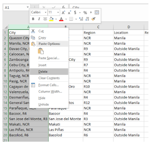
You can now discard the data in column A by right-clicking on the column header 

and selecting Delete from the menu:

The data in column A is removed and the remaining data shifts one column to the 

left. Note that the cell references in your formulas have changed to the new column 

letters automatically:

Get the Average Revenue.

Get the Highest Revenue.

Get the Lowest Revenue.