Data Analytics for Business.: KPI IN EXCEL : Focus on Operating Profit %

Key performance indicators (KPIs) are visual measures of performance and usually included in reports. Supported by a specific calculated field, a KPI is designed to help users quickly evaluate the current value and status of a metric against a defined target.

In this blog, we will use Operating Profit % as a KPI since Small and Medium enterprises need to understand that Operating profit is a useful and accurate indicator of a business's health.

Here's how to use KPI in Excel. Open the data "KPI Data" from Github https://github.com/alcadelina/KPI

Step 1. Open an Excel file. Click on the File tab on the uppermost ribbon. Go to Options.

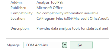
Step 2: Under Options > Click on Add-ins. You’ll be able to see the screen as shown below.

Step 3: Select COM Add-ins under the Manage section dropdown and click on the Go button.

Step 4: As soon as you hit the Go button, the COM Add-ins dialog box will pop up. Select Microsoft Power Pivot for Excel from the list of add-ins and click OK.

After enabling this PowerPivot add-in, you should be able to see the PowerPivot option tab on the topmost panel ribbon in your excel.

Step 5: Under the PowerPivot tab in your excel file, click on Manage.

Step 6: It should open a new tab named Power Pivot for Excel.
Step 7: Once you click on the “From Other Sources” tab, a new window named Table Import Wizard will pop up. There you can see a lot of options from where you can import the data to PowerPivot. Select the Excel file, then click on the Next button to proceed further.

Step 8: Browse the path on where your excel data file is stored and click the Next button to finish the Import.

Step 9: Click on the Finish button once the data table is loaded into PowerPivot.

Step 10: After a successful import, you will be able to see the data as below.

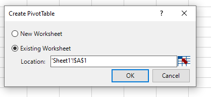
Step 11: Now, in order to create a KPI report, we need to slice and dice our data under the pivot table. Click on the Pivot Table tab under PowerPivot. Once you click it, a new window named Create PivotTable will appear in which you have to select the data from PowerPivot, and it asks you whether you want a pivot table under a new sheet or on the same sheet. I will prefer to go with the same sheet and then will provide the range on which the pivot table should be added. Click OK once done.

Step 12: Select the data under rows, columns, and values, as shown below.

Here we have selected data in the following order:

Rows: Accounting Date Year & Quarter

Values: Sum of Total Sales & Operating Profit

Step 13: Now, we are going to add a calculated column in the pivot. Select Measures under excel sheet. Click on New Measures.

A new window called Measure will pop up. It will allow you to formulate a measure and add it under your pivot table created.

Step 14: Under ” Measure name:”, add a name OPERATING PROFIT %. If you want to add a description for the same, you can add it there as well under the Description section. In this case, Operating Profit Percentage measures how much of a profit the company is generating from their main operations. The operating profit percentage represents the percentage of a company’s sales that ultimately end up as profit.

Under the Formula section, add the formula =[Sum of Operating Profit]/[Sum of Total Sales] as shown below. It will calculate the OPERATING PROFIT % for you. See the screenshot below.

Above, we have created a new calculated column named Operating Profit %, which can be formulated as the ratio of two columns, Sum of Operating Profit and Sum of Total Sales.

Step 15: Select the entire column, Operating Profit %, and convert it to % using number formatting.

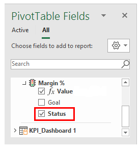
Step 16: Now our data is ready for KPI’s to be added. Click on the KPIs tab as shown in the figure. Select the New KPI option.

A KPI window will pop up, as shown below. It has some by default values, which we are going to change.

Step 17: In this window, define an Absolute Value for the target as 1. We are doing this because we don’t have any other target values/measures defined as separately to have a comparison with actual values of Operating Profit %.

Step 18: In this step, define the Status Threshold value. It is defined in decimal format. Like 30% will be given as 0.30. Change the Status Threshold values as shown in the screenshot above. Make the right one 0.3.

Step 19: Now, we can select icon style as well (These are the KPI Icons). I will opt out of the second style. As shown below.