Excel Data Cleaning Techniques: Separate First, Middle, and Last Names Using Formulas; Duplicate Detection and Removal

Separate First, Middle, and Last Names Using Formulas 

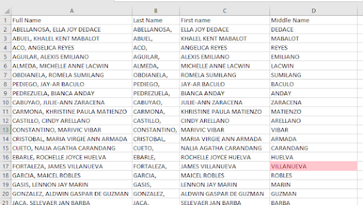
Suppose you have the dataset as shown below and you want to quickly separate the first, last, and middle names in one cell.

The below formula will give you the first name:

=LEFT(A2,SEARCH(" ",A2)-1)

The above formula uses the SEARCH function to get the position of the space character in between the first and last name. The LEFT function then uses this space position number to extract all the text before it.

2. Get the Last Name by going to cell B2 and typing = LEFT(A2,SEARCH(" ",A2)-1)

3. Get the First Name by typing in cell C2 =RIGHT(A2,LEN(A2)-SEARCH(" ",A2))

4. Get the Middle Name by typing in cell D2 =RIGHT(A2,LEN(A2)-SEARCH("@",SUBSTITUTE(A2," ","@",LEN(A2)-LEN(SUBSTITUTE(A2," ","")))))

Finding Duplicates

There can be 2 things you can do with duplicate data – Highlight It or Delete It. It is possible to find duplicate data in Excel and to highlight them. The following example demonstrates the process of finding duplicate data in Excel.

1. Select the range of the data in which duplicates are to be searched for. In this case, cells A1:B38 have been selected.

2. Go to Home > Styles > Conditional Formatting.

3. Choose the option Highlight Cells Rules. Then click on Duplicate Values.

4. Select a formatting style. Click OK.

Result: The duplicate names are highlighted.

Removing Duplicates

Upon finding the duplicate data, Excel can also remove them. The following example illustrates the process.

1. Select any specific cell within the data set selection.

2. Go to Data tab > Data Tools. Then click on Remove Duplicates.

The dialog box appears.

3. Check on all the checkboxes and then click OK.

Result: Excel omits all duplicate rows whilst keeping the first one intact.

Excel Forecast sheet: Forecasting the 2021 Pag-IBIG 2 Dividend Rate

 

If you have historical time-based data, Excel Forecast Sheet can help you create a forecast by creating a new worksheet that contains both a table of the historical and predicted values and a chart that expresses this data. A forecast can help data analysts predict things like future sales, inventory requirements, or consumer trends.

Forecast Sheet can be found in Excel for Microsoft 365, Excel 2021, Excel 2019, and Excel 2016. 

Let us have the Pag-IBIG 2 Dividends as an example. The Modified Pag-IBIG II (Pag-IBIG MP2) Savings Program is a special and voluntary savings facility with a 5-year maturity, designed for active Pag-IBIG Fund members who wish to save more and earn even higher dividends, in addition to their Pag-IBIG Regular Savings. Every March, Pag-BIG Fund announces the dividend rate earned by members, and in 2020 it was 6.12%.

Our goal is to forecast the 2021 Pag-IBIG 2 Dividend Rate,

1. Select the range of cells containing the target data.

2. From the ribbon, go to Data > Forecast > Forecast Sheet.

3. Select the chart and in the Chart Elements include Data Labels.

4. The forecast shows the Pag-IBIG 2, 2021 Dividend Rate is 6.3% with lower confidence of 4.61% and upper confidence of 8%.

Let us see in March 2021, if the Pag-IBIG 2 dividend rate will range between 4.61% and 8% and whether 6.3% is fairly accurate.

Excel Data Cleaning Techniques: Handling Blank Cells

 

Blank cells might occur among a large set of data and can cause a lot of trouble to the user. Blank cells can create havoc if not treated beforehand. I often face issues with blank cells in a data set that is used to create reports/dashboards.

You may want to fill all blank cells with ‘0’ or ‘Not Available’, or may simply want to highlight it. If there is a huge data set, doing this manually could take hours. Thankfully, there is a way you can select all the blank cells at once. 

Finding blank cells is a tedious job if done manually. But Excel has a great way of selecting all blank cells in a given data set simultaneously. The blank cells can be simply highlighted or marked with a certain symbol. The following example shows the method of selecting all blank cells at once.

1. Select the complete data set.

2. Go to Home > Editing > Find & Select > Go To Special.

3. Select Blanks. Then click OK.

In this way, all blank cells in the data set are selected. Inputs such as 0, Absent, or Not Available can be inserted in such blank cells, only by typing the desired text and pressing CTRL+Enter.

Excel Data Cleaning Techniques: Getting Rid of Extra Spaces

    Excel Data Cleaning is a significant skill that all Business and Data Analysts must possess. In the current era of data analytics, everyone expects the accuracy and quality of data to be of the highest standards. A major part of Excel Data Cleaning involves the elimination of blank spaces, incorrect, and outdated information.  Data cleaning in MS Excel includes many variants, such as removal of extra or blank spaces and duplicate data, changing text to upper or lower case, converting stored text into numbers, highlighting errors, spell check, parsing data, etc. Five amazing data cleaning techniques will be shared and I will start today with Getting Rid of Extra Spaces.

    The TRIM function is used to eliminate excess spaces and tab spaces in the Excel worksheet cells. The excessive blank spaces and tab spaces make the data hard to understand. Using the "TRIM" function can eliminate these excessive blank spaces.

Excel allows us to use the TRIM function to omit extra spaces in between texts, as well as before or after texts.

Syntax: =TRIM(text)

The TRIM function takes in a cell reference (or text) as input. The function omits any spaces before, after, or in between the text (except single spaces between words).

Select the data cells with excessive blank spaces and tab spaces. Now, select a new cell adjacent to the first cell.

Apply the TRIM() function and drag the cell as shown below.

It shows the final data after the elimination of the excess space as follows.

Excel: Forecasting using Exponential Triple Smoothing

The Excel FORECAST.ETS function uses the AAA version of the advanced machine learning Exponential Triple Smoothing (ETS) algorithm to forecast future values based on historical data.

The FORECAST.ETS function is available in Excel 2016 or later versions. This function can detect a seasonal pattern of data.

1. The function predicts a future value by Exponential Triple Smoothing.

Let us have an example:

Providing the last three arguments is not mandatory. The fourth argument defines the size of the seasonal pattern. A default value of 1 implies that the seasonality is automatically found.

2. Enter 1350 in the cell C. Select the cells A1:C11. Create a scatter plot with straight lines and markers.

3. The function FORECAST.ETS.SEASONALITY can be used to find the length of the seasonal pattern.

Excel Forecasting using Linear Regression.

 Excel Forecasting using Linear Regression.

Excel allows us to predict missing or future data based on a given set of data. Excel follows a linear trend to forecast data using the FORECAST function. The new FORECAST.LINEAR function is a new Excel function for forecasting and the function FORECAST.LINEAR can predict a future value in a linear fashion.

The FORECAST.LINEAR function is categorized under Excel Statistical functions. It will calculate or predict a future value using linear regression.

In financial modeling, the FORECAST.LINEAR function can be useful in calculating the statistical value of a forecast made. For example, if we know the past earnings and expenses that are a certain percentage of sales, we can forecast the future amounts using the function.

Let us have an example:

Objective: Forecast the demand on day 8 to 10 using linear regression.

Step 1. Go to cell C8 and type =FORECAST.LINEAR(A8,B2:B7,A2:A7)

Step 2. By dragging the FORECAST.LINEAR function downwards, the absolute references ($B$2:$B$7 and $A$2:$A$7) remain fixed. However, the relative reference cell (A8) changes to A9 and A10.

Step 3. Enter 1350 into cell C7. Select the cells A1:C11. Create a scatter plot with straight lines and markers.

Step 4. Select Scatter Plots with Straight Lines and Markers.

When a trendline is added to a chart, the equation can be displayed. The equation can extrapolate future values based on the given data.

Step 5. Change Chart Style that fits your intended audience.

Final result of the Forecast using Linear Regression.

TABLEAU ONLINE: CATALOG