SAMPLING: SAMPLING ACCOUNTS RECEIVABLE

 This Business Analytics lecture tackles Random Sampling. The data Random Accounts Receivable IN PESO.xlsx is available at https://github.com/alcadelina/business-analytics-excel-data.

We want to choose a random size of 25 and do it 25 random sample times in the 280 accounts.

How can this be possible? And how do we calculate the average amount owed in each random sample and create the histogram using Tableau.

Objective: Demonstrate how sample means are distributed.

Excel Solution:

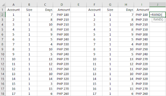
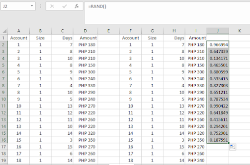
Step 1. Random numbers next to a copy.  Copy the original data to columns F.G.H.I. Then enter the formula: =RAND() in cell J1 and copy it down column J.

Step 2. Replace with values. To enable sorting, you must first “freeze” the random numbers ----that is replace their formulas with values. To do this, copy the range J1:J280 and select Paste values from the Paste dropdown menu on the Home Ribbon.

Step 3. Sort. Sort on Column J in ASCENDING ORDER.  Then the 25 smallest random numbers are the ones in the sample.

 Step 4. Repeat Steps 2 and 3,  25 TIMES. Copy the values in Cell I in a new worksheet.

Step 5. Make a Table similar below. Use the Average Cost for Histogram.

Step 6. Then do the Histogram Using Tableau.

Step 7. Create Annotation for your Insights. 

Arnel Lopez Cadeliña, MBA, REA, CFA (Investment Foundation Certificate)

BUSINESS INTELLIGENCE TOOL FOR DATA ANALYSIS

The file Baseball Salaries with Team Info3. xlsx contains a sheet for each year from 2012 to 2018 listing each player, his team, his position, and his salary for that year. It also contains a Teams sheet that lists each team, the division and league of the team, and the team's city, state/province, and country.

The file can be downloaded at https://github.com/alcadelina/business-analytics-excel-data. 

Objective: To learn the mechanics of Tableau public for creating a viz of baseball team salaries.

The output should be similar below:

Step 1. Upload the Team Info3. xlsx to Tableau Desktop. 

Step 2. Drag "Year" to Columns Pill, Make sure it is Discrete and in color blue. Drag "Salary" to Rows pill. Drag "Team" to Color and into "Detail" in the Marks Card. Explore how to highlight Los Angeles Dodgers. Name your Sheet "Team salaries per Year".

Step 3. In a new Sheet, Drag "Year" to Columns Pill, Make sure it is Discrete and in color blue. Drag "Salary" to Rows pill.Drag "Team" to Color and into "Detail" in the Marks Card. Filter the "Division" choose only "National West", filter the "Position" choose only "Pitcher".Explore how to highlight Los Angeles Dodgers. Name your Sheet "National West Teams salaries of Pitchers per Year".

Step 4. In a new sheet, drag Longitude to "Columns" pill and Latitude to "Rows" pill. Drag " Country", "State,Province" and " City" to Colors in the Marks Card. Drag "Salary" to size. Adjust if necessary. rag " Country", "State,Province" , " City" and "Salary" to Detail in the Marks card. Explore how to highlight Los Angeles Dodgers. Name your Sheet "Team Salary Map".

Step 5. Create a dashboard using your sheets. Adjust margins and padding. The output should be similar below:

Arnel Lopez Cadeliña, MBA, REA, CFA (Investment Foundation Certificate)

BINOMIAL DISTRIBUTION USING EXCEL AND TABLEAU

 

The point of this example is that if each mutual fund has a 50-50 chance of beating the market in any given week, it is very unlikely for a particular mutual fund to beat the market in at least 37 out of 52 weeks. However, if you have a lot of such mutual funds, then it is fairly likely that at least one of them will beat the market this often.  You can see this from the data table. For example, if there are 600 mutual funds, the chance of at least one beating the market at least 37 out of 52 weeks is greater than 60%.

An analogy might help. If a person flips a coin 100 times, it's not very likely that she will get a streak of, say, 10 heads in a row. But if hundreds of people flip a coin 100 times, it's almost certain that at least one of them will get such a streak.

An Investment broker at Vizee Analytics claims that he has found a real winner. He has tracked a mutual fund that has beaten a standard market index in 37 of the past 52 weeks. Could this be due to chance, or has he really found a winner?

Objective: To determine the probability of a mutual fund outperforming a standard market index at least 37 out of 52 weeks.

The broker is no doubt tracking many mutual funds and he is only reporting only the vest if these. Rgere is a 50-50 chance of beating the market index, independently of performance in other weeks. In other words, rge number of weeks where the given fund outperforms the market index is binomially distributed with n=52 and p=0.5. The probability is P(X >  37) = 1 -P (x < 36) the relevant formula is:

=1-BINOM.DIST(B3-1,B4,0.5,TRUE)

To see whether any of the 400 funds beat the market at least 37 of 52 weeks , calculate P( Y >  1) = 1 -P (Y=0) in cell B9 with the formula:

=1-BINOM.DIST(0,B8,B6,TRUE)

The data shows beating the market 37 times out of 52 is no big deal with 400 funds, but beating it 40 times out of 52 even with 600 funds. The probability of this happening purely by chance is only 0.038 or less than 1 out of 25.

To see how the probability in cell B9 depends on the level of success on the reported fund (the value in cell B3) and the number of mutual funds being tracked 9ib cell B8), a two-way data table has been created in the range B13:G18. The formula in cell B13 is =B9, the row input cell is B3 and the column input cell is B8).

The Excel data for  Tableau:

SAMPLING: SAMPLING FAMILIES TO ANALYZE ANNUAL INCOMES

 In this Business Analytics lecture tackles about Random Sampling. The data Random Sampling.xlsm is available at https://github.com/alcadelina/business-analytics-excel-data. The extension is .xlsm because the file contains macro hence when you open it you have to enable it. 

We want to choose a simple random sample size of 10 out of the 40 population.

How can this be possible? And how do the summary statistics of the chosen families compare to the corresponding summary statistics of the population?

Objective: To illustrate how Excel’s random number function, RAND, can be used to generate simple random samples.

Excel Solution:

Step 1. Random numbers next to a copy.  Copy the original data to columns D and E. Then enter the formula: =RAND() in cell F10 and copy it down column F.

Step 2. Replace with values. To enable sorting, you must first “freeze” the random numbers ----that is replace their formulas with values. To do this, copy the range F10:F49 and select Paste values from the Paste dropdown menu on the Home Ribbon.

Step 3. Sort. Sort on Column F in ASCENDING ORDER.  Then the 10 families with the 10 smallest random numbers are the ones in the sample.

Step 4. Use the AVERAGE, MEDIAN, AND STDEV.S Functions in Row 6 to calculate summary statistics of the first 10 incomes in Column E. Similar summary statistics for the population have already been calculated in Row 5. (cell D5 uses STDEV.P function because this is the POPULATION standard Deviation)

For the Population Mean:

For the Population Median:

For the Population Standard Deviation:

For Sample Mean:

For Sample Median:

For sample Standard Deviation:

So the complete Excel data is:

You now have 10 sample size out of the 40 population using  simple random sampling.

Practice set.

Use the data “Practice Random Sampling” from https://github.com/alcadelina/business-analytics-excel-data . Generate 20 sample size out of 204 population.

Arnel Lopez Cadeliña, MBA, REA, CFA (Investment Foundation Certificate)

 

PROBABILITY DISTRIBUTION : MARKET RETURN SCENARIOS FOR THE NATIONAL ECONOMY

 In this Business Analytics lecture, the Market Return.xlsx data is available at https://github.com/alcadelina/business-analytics-excel-data

As a Business Manager, you are concerned with the market return for the coming year, where the market return is defined as the percentage gain (or loss, if negative) over the year. You believe there are 5 possible scenarios for the national economy in the coming year:

    Scenario                                         Estimated Market Return    Probability

1. Rapid Expansion                           23%                                        0.12

2. Moderate Expansion                     18%                                        0.40

3. No Growth                                    15%                                        0.25

4. Moderate Contraction                    9%                                         0.15

5. Serious Contraction                       3%                                         0.08

The objective is to compute the Mean, Variance, and Standard Deviation of the probability distribution of the market return for the coming year using Excel and visualize the Simulation in Density using Tableau..

Solution for Excel.

To make the connection between the general notation, let X denote the market return for the coming year. Then each possible economic scenario leads to a possible value of X. 

Step 1. Mean Return. Calculate the mean return in cell B11 with the formula:

=SUMPRODUCT(C4:C8,B4:B8)

Step 2. Squared Deviations. to get ready to compute the variance, calculate the squared deviations from the mean by entering the formula

= (C4-Mean)^2

in cell D4 and copying it down through cell D8.

Step 3. Variance. Calculate the variance of the market return in cell B12 with the formula

= SUMPRODUCT(Sq_dev_from_mean,Probability)

=SUMPRODUCT(Market_return,Market_return,Probability)-Mean^2

Step 4. Standard Deviation. calculate the Standard deviation of the Market return in cell B13 with the formula

=SQRT(Variance)

Step 5. we will do Simulation. Create a 2nd worksheet and name it SIMULATION. Then copy the details below. Also copy the Average Return and Std.Dev return from the original sheet.

In your Look Up table copy the "Return" and do the Cum Probability

Step 6. On the "Simulation" type the formula of RAND as show below:

Step 7. Type the VLOOKUP Formula as shown below:

Step 8. On the "Summary statistics from simulation below" , type the Average formula as shown below:

and the Std. Dev of returns as shown below:

Below is the complete Excel Output.

In tableau, Visualize the Market return using density:

Arnel Lopez Cadeliña, MBA, REA, CFA (Investment Foundation Certificate)